Evaluating iterative algorithms

Many generative methods (e.g., genetic algorithms) iteratively explore sequences to improve sequence fitness. In this notebook, we show on toy sequences how to evaluate sequences optimized across multiple rounds and visualize the results using seqme.

import seqme as sm

Single run

seqme allows naming sequence entries as a tuple. Here we name an entry using the following format: (model name, iteration).

sequences = {
    ("model 1", 1): ["QLF", "FFQLL", "RQLL"],
    ("model 1", 2): ["RQLF", "PRFQRP", "RQLL"],
    ("model 1", 3): ["RQLRR", "RQLRRR", "RQLRRR"],
    ("model 2", 1): ["QLF", "QLF", "RQLL"],
    ("model 2", 2): ["QLF", "FFQRP", "RQLL"],
    ("model 2", 3): ["PLFR", "RFQRP", "RQLR"],
}

Let’s define the metrics to compute.

metrics = [
    sm.metrics.ID(predictor=sm.models.Charge(), name="Charge", objective="maximize"),
    sm.metrics.ID(predictor=sm.models.Hydrophobicity(), name="Hydrophobicity", objective="maximize"),
    sm.metrics.Uniqueness(),
]

Let’s compute the metrics.

df = sm.evaluate(sequences, metrics)

100%|██████████| 18/18 [00:00<00:00, 793.34it/s, data=('model 2', 3), metric=Uniqueness]    

sm.show(df, color_style="bar", caption="Table 1.1 Iterative algorithms")

Table 1.1 Iterative algorithms

		Charge↑	Hydrophobicity↑	Uniqueness↑
model 1	1	0.33±0.34	0.32±0.32	1.00
	2	1.33±0.34	-0.43±0.16	1.00
	3	3.66±0.34	-1.57±0.06	0.67
model 2	1	0.33±0.34	0.23±0.26	0.67
	2	0.66±0.34	0.01±0.24	1.00
	3	1.66±0.34	-0.70±0.36	1.00

Let’s highlight it differently.

sm.show(df, color_style="bar", caption="Table 1.2 Iterative algorithms", level=1)

Table 1.2 Iterative algorithms

		Charge↑	Hydrophobicity↑	Uniqueness↑
model 1	1	0.33±0.34	0.32±0.32	1.00
	2	1.33±0.34	-0.43±0.16	1.00
	3	3.66±0.34	-1.57±0.06	0.67
model 2	1	0.33±0.34	0.23±0.26	0.67
	2	0.66±0.34	0.01±0.24	1.00
	3	1.66±0.34	-0.70±0.36	1.00

Notice in the above table visualization, we set level=1, this means that each sub metric dataframe (model 1 and model 2) should be colored, underlined and bolded, independently.

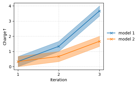
Let’s visualize the sequences performance at each step.

sm.plot_line(df, metric="Charge")

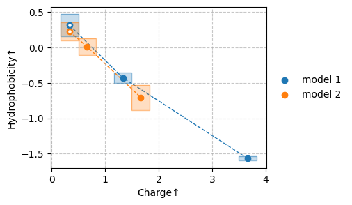
Let’s look at two metrics.

sm.plot_scatter(df, metrics=["Charge", "Hydrophobicity"])

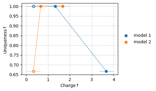
sm.plot_scatter(df[["Charge", "Uniqueness"]])

Let’s sort the sequences by their charge.

df2 = sm.sort(df, "Charge", level=0)
sm.show(df2, caption="Table 2.1. Iterative algorithms (sorted)", color_style="bar", hline_level=0)

Table 2.1. Iterative algorithms (sorted)

		Charge↑	Hydrophobicity↑	Uniqueness↑
model 1	3	3.66±0.34	-1.57±0.06	0.67
model 2	3	1.66±0.34	-0.70±0.36	1.00
model 1	2	1.33±0.34	-0.43±0.16	1.00
model 2	2	0.66±0.34	0.01±0.24	1.00
model 1	1	0.33±0.34	0.32±0.32	1.00
model 2	1	0.33±0.34	0.23±0.26	0.67

Let’s rearrange the entries levels and sort the sequence by uniqueness within each iteration.

df3 = df.reorder_levels([1, 0])
df3 = sm.sort(df3, "Uniqueness", level=1)

sm.show(
    df3, color="#d668c9", caption="Table 2.2. Iterative algorithms (sorted within iteration)", color_style="gradient"
)

Table 2.2. Iterative algorithms (sorted within iteration)

		Charge↑	Hydrophobicity↑	Uniqueness↑
1	model 1	0.33±0.34	0.32±0.32	1.00
	model 2	0.33±0.34	0.23±0.26	0.67
2	model 1	1.33±0.34	-0.43±0.16	1.00
	model 2	0.66±0.34	0.01±0.24	1.00
3	model 2	1.66±0.34	-0.70±0.36	1.00
	model 1	3.66±0.34	-1.57±0.06	0.67

Let’s display the sequences with largest charge in each iteration.

df4 = df.reorder_levels([1, 0]).sort_index()
df4 = sm.top_k(df4, "Charge", k=1, level=1)
sm.show(df4, color_style="bar", hline_level=0, caption="Table 2.3. Best per iteration")

Table 2.3. Best per iteration

		Charge↑	Hydrophobicity↑	Uniqueness↑
1	model 1	0.33±0.34	0.32±0.32	1.00
	model 2	0.33±0.34	0.23±0.26	0.67
2	model 1	1.33±0.34	-0.43±0.16	1.00
3	model 1	3.66±0.34	-1.57±0.06	0.67

Multiple runs

Let’s assume we ran two generative models multiple times with a different seed each time. The sequences from the runs are shown below. And now we want to compute the deviation in performance across runs.

sequences_run1 = {
    ("model 1", 1): ["QLF", "FFQLL", "RQLL"],
    ("model 1", 2): ["RQLF", "PRFQRP", "RQLL"],
    ("model 1", 3): ["RQLRR", "RQLRRR", "RQLRRR"],
    ("model 2", 1): ["QLF", "FFQRP", "RQLL"],
    ("model 2", 2): ["QLF", "FFQRP", "RQLL"],
    ("model 2", 3): ["PLFR", "RFQRP", "RQLR"],
}

sequences_run2 = {
    ("model 1", 1): ["QLF", "FFQLL", "RQLL"],
    ("model 1", 2): ["RQLF", "PRFQRP", "RQLL"],
    ("model 1", 3): ["RQLRR", "RQLRRR", "RQLRRR"],
    ("model 2", 1): ["QLF", "FFQRP", "RQLL"],
    ("model 2", 2): ["QLF", "FFQRP", "RQLL"],
    ("model 2", 3): ["PLFR", "RFQRP", "RQLR"],
}

sequences_run3 = {
    ("model 1", 1): ["RQLF", "PRFQRP", "RQLL"],
    ("model 1", 2): ["QLF", "FFQLL", "RQLL"],
    ("model 1", 3): ["RQLRR", "RQLRRR", "RQLRRR"],
    ("model 2", 1): ["QLF", "FFQRP", "RQLL"],
    ("model 2", 2): ["QLF", "FFQRP", "RQLL"],
    ("model 2", 3): ["PLFR", "RFQRP", "RQLR"],
}

sequences_per_run = [sequences_run1, sequences_run2, sequences_run3]

Let’s define the metrics to compute.

metrics = [
    sm.metrics.ID(predictor=sm.models.Charge(), name="Charge", objective="maximize"),
    sm.metrics.Uniqueness(),
]

df_per_run = [sm.evaluate(sequences, metrics) for sequences in sequences_per_run]

100%|██████████| 12/12 [00:00<00:00, 2110.78it/s, data=('model 2', 3), metric=Uniqueness]
100%|██████████| 12/12 [00:00<00:00, 3515.03it/s, data=('model 2', 3), metric=Uniqueness]
100%|██████████| 12/12 [00:00<00:00, 3198.50it/s, data=('model 2', 3), metric=Uniqueness]

Let’s create a metric dataframe combining the metric dataframe of each run.

df_combined = sm.combine(df_per_run, value="mean", deviation="se")

Let’s rank the models using all the metrics.

df_combined = sm.rank(df_combined, tiebreak="mean-rank")

sm.show(df_combined, color="#6892d6", color_style="bar", caption="Table 3.1. Multiple runs", n_decimals=[2, 2, 0])

Table 3.1. Multiple runs

		Charge↑	Uniqueness↑	Rank↓
model 1	1	0.66±0.34	1.00±0.00	4
	2	1.00±0.34	1.00±0.00	3
	3	3.66±0.00	0.67±0.00	2
model 2	1	0.66±0.00	1.00±0.00	4
	2	0.66±0.00	1.00±0.00	4
	3	1.66±0.00	1.00±0.00	1

Let’s extract the top two ranked entries.

sm.show(
    sm.top_k(df_combined, "Rank", 2),
    color="#6892d6",
    color_style="bar",
    caption="Table 3.2. Multiple runs - Best",
    n_decimals=[2, 3, 0],
)

Table 3.2. Multiple runs - Best

		Charge↑	Uniqueness↑	Rank↓
model 1	3	3.66±0.00	0.667±0.000	2
model 2	3	1.66±0.00	1.000±0.000	1

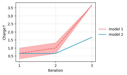
Let’s visualize the sequences performance at each iteration.

sm.plot_line(df_combined, "Charge", color=["#ff4949ff", "#29a1c6ff"], linestyle=["--", "-"], marker=None)