Getting started

In this notebook, we show how to use seqme to evaluate biological sequences and add your own metric. We introduce seqme’s functionality through toy examples. Other tutorials show real-world use cases.

First the imports.

from pprint import pprint
from typing import Literal

import numpy as np

import seqme as sm

Basics

Let’s define the sequences to use and the metrics to compute. Some sequences will be loaded from fasta files, others are hard-coded.

First let’s write a fasta file with random sequences to disk.

RANDOM_SEQUENCES_PATH = "./data/random.fasta"

random_sequences = ["KKKKK", "PLQ", "RKSPL"]

sm.to_fasta(random_sequences, RANDOM_SEQUENCES_PATH)

UniProt contains a lot of sequences. To speed-up the metric computations, we will only use a (random) subset of the UniProt sequences.

sequences = {
    "Random": sm.read_fasta(RANDOM_SEQUENCES_PATH),
    "UniProt": sm.utils.subsample(["KKWQ", "RKSPL", "RASD"], n_samples=2, seed=42),
    "HydrAMP": ["MMRK", "RKSPL", "RRLSK", "RRLSK"],
    "hyformer": ["MKQW", "RKSPL"],
}

Metrics may precompute some values upon metric object creation to speed up the overall process.

def hit_rate_condition_fn(sequences: list[str]) -> np.ndarray:
    no_lysine = ~np.array(["K" in seq for seq in sequences])
    return no_lysine


def my_embedder(sequences: list[str]) -> np.ndarray:
    lengths = [len(sequence) for sequence in sequences]
    counts = [sequence.count("K") for sequence in sequences]
    return np.array([lengths, counts], dtype=float).T


metrics = [
    sm.metrics.Uniqueness(),
    sm.metrics.Novelty(reference=sequences["UniProt"], name="Novelty (UniProt)"),
    sm.metrics.Diversity(),
    sm.metrics.FBD(reference=sequences["Random"], embedder=my_embedder),
    sm.metrics.ID(sm.models.Gravy(), name="Gravy", objective="minimize"),
    sm.metrics.HitRate(condition_fn=hit_rate_condition_fn),
]

Let’s compute the metrics.

df = sm.evaluate(sequences, metrics)

 38%|███▊      | 9/24 [00:00<00:00, 289.30it/s, data=UniProt, metric=FBD]              /Users/rasmus.larsen/work/hackathon-2025/seqme/src/seqme/metrics/fbd.py:91: LinAlgWarning: Matrix is singular. The result might be inaccurate or the array might not have a square root.
  covmean = scipy.linalg.sqrtm(sigma1.dot(sigma2))
100%|██████████| 24/24 [00:00<00:00, 614.03it/s, data=hyformer, metric=Hit-rate]         

Let’s look at the results.

df

	Uniqueness		Novelty (UniProt)		Diversity		FBD		Gravy		Hit-rate
	value	deviation	value	deviation	value	deviation	value	deviation	value	deviation	value	deviation
Random	1.00	NaN	1.0	NaN	0.866667	NaN	0.000000	NaN	-1.911111	1.032855	0.333333	0.272166
UniProt	1.00	NaN	0.0	NaN	1.000000	NaN	3.961130	NaN	-2.400000	0.650000	0.500000	0.353553
HydrAMP	0.75	NaN	1.0	NaN	0.700000	NaN	8.602244	NaN	-1.627500	0.209816	0.000000	0.000000
hyformer	1.00	NaN	1.0	NaN	0.800000	NaN	8.228118	NaN	-1.500000	0.100000	0.000000	0.000000

… let’s make it nicer to look at.

sm.show(df, n_decimals=2)

	Uniqueness↑	Novelty (UniProt)↑	Diversity↑	FBD↓	Gravy↓	Hit-rate↑
Random	1.00	1.00	0.87	0.00	-1.91±1.04	0.33±0.28
UniProt	1.00	0.00	1.00	3.96	-2.40±0.65	0.50±0.36
HydrAMP	0.75	1.00	0.70	8.60	-1.63±0.21	0.00±0.00
hyformer	1.00	1.00	0.80	8.23	-1.50±0.10	0.00±0.00

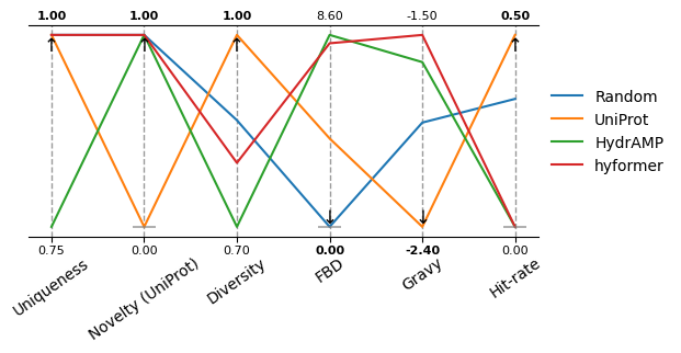
Let’s also do a parallel coordinates plot.

sm.plot_parallel(df, arrow_size=12, xticks_fontsize=10, xticks_rotation=35, figsize=(6, 2.5), show_arrow=False)

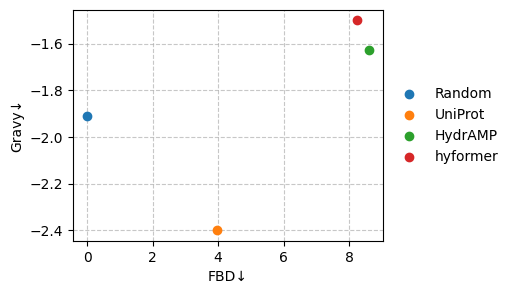
We are particularly interested in the following two metrics.

sm.plot_scatter(df, metrics=["FBD", "Gravy"], show_deviation=False)

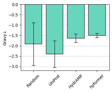
Let’s zoom in on one of the metrics.

sm.plot_bar(df, "Gravy")

Let’s extract the two rows with lowest Gravy.

sm.show(sm.top_k(df, "Gravy", k=2))

	Uniqueness↑	Novelty (UniProt)↑	Diversity↑	FBD↓	Gravy↓	Hit-rate↑
Random	1.00	1.00	0.87	0.00	-1.91±1.04	0.33±0.28
UniProt	1.00	0.00	1.00	3.96	-2.40±0.65	0.50±0.36

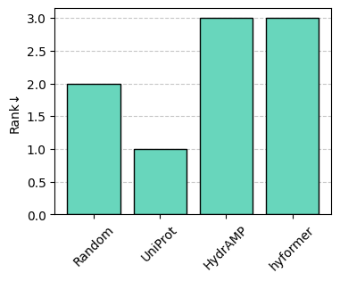
Let’s perform a (non-dominated) ranking of the entries, which corresponds to computing slices of the Pareto front from the selected metrics, followed by removing the entries in the current slice. Each slice corresponds to a rank.

df = sm.rank(df, metrics=["Hit-rate", "Diversity", "Gravy"])

Let’s plot the ranking.

sm.plot_bar(df, "Rank")

To write a metric dataframe to disk, encode the dataframe as a pickle object.

PATH = "./metrics_dataframe.pkl"

sm.to_pickle(df, PATH)
sm.show(sm.read_pickle(PATH), color_style="gradient")

	Uniqueness↑	Novelty (UniProt)↑	Diversity↑	FBD↓	Gravy↓	Hit-rate↑	Rank↓
Random	1.00	1.00	0.87	0.00	-1.91±1.04	0.33±0.28	2.00
UniProt	1.00	0.00	1.00	3.96	-2.40±0.65	0.50±0.36	1.00
HydrAMP	0.75	1.00	0.70	8.60	-1.63±0.21	0.00±0.00	3.00
hyformer	1.00	1.00	0.80	8.23	-1.50±0.10	0.00±0.00	3.00

It is also possible to export the dataframe to a LaTeX table or a PNG as shown below.

To save the styled metric dataframe to a png, we use dataframe_image.

# !pip install dataframe_image

SAVE_TABLE = False

if SAVE_TABLE:
    # save to LaTeX
    sm.to_latex(df, "table.tex", n_decimals=3, color=None, caption="My first table")

    # save to PNG
    import dataframe_image as dfi

    styler = sm.show(df, n_decimals=3, color_style="bar")
    await dfi.export_async(styler, "table.png", dpi=300)

That it all for the basic usage of seqme. Check out the documentation for the metrics and models implemented in seqme.

Let’s now look at some more advanced features!

Advanced

In the advanced section, we show how to

• Combine multiple metric dataframes into one.

• Improve performance through caching.

• Create your own metric.

Combining metric dataframes

seqme’s combine can combine metric dataframes with different sequences and/or metrics. This can be useful if you want to evaluate the sequences on an additional metric or add an additional set of sequences for evaluation - without needing to recompute the results.

Let’s create three metric dataframes.

df1 = sm.evaluate(
    sequences={
        "s1": ["KKKKK", "PLUQ", "RKSPL"],
        "s2": sm.utils.subsample(["KKWQ", "RKSPL", "RASD"], n_samples=2, seed=42),
        "s3": ["MMRK", "RKSPL", "RRLSK"],
        "s4": ["MKQW", "RKSPL"],
    },
    metrics=[
        sm.metrics.Novelty(reference=["KKW", "RKSPL"]),
        sm.metrics.Novelty(reference=["RASD", "KKKQ", "LPTUY"], name="Novelty (Random)"),
    ],
    verbose=False,
)

df2 = sm.evaluate(
    sequences={"s4": ["MKQW", "RKSPL"], "s5": ["MKQW"]},
    metrics=[sm.metrics.ID(sm.models.Gravy(), name="Gravy", objective="minimize")],
    verbose=False,
)

df3 = sm.evaluate(
    sequences={"s6": ["MKQW", "RKSPL"]},
    metrics=[
        sm.metrics.ID(sm.models.Gravy(), name="Gravy", objective="minimize"),
        sm.metrics.Novelty(reference=["KKW", "RKSPL"]),
    ],
    verbose=False,
)

Let’s combine the dataframes.

df = sm.combine([df1, df2, df3])

df

	Novelty		Novelty (Random)		Gravy
	value	deviation	value	deviation	value	deviation
s1	0.666667	NaN	1.0	NaN	NaN	NaN
s2	1.000000	NaN	0.5	NaN	NaN	NaN
s3	0.666667	NaN	1.0	NaN	NaN	NaN
s4	0.500000	NaN	1.0	NaN	-1.5	0.1
s5	NaN	NaN	NaN	NaN	-1.6	NaN
s6	0.500000	NaN	NaN	NaN	-1.5	0.1

… let’s make it nicer to look at.

sm.show(df, n_decimals=[3, 2, 1], color="#d66868")

	Novelty↑	Novelty (Random)↑	Gravy↓
s1	0.667	1.00	-
s2	1.000	0.50	-
s3	0.667	1.00	-
s4	0.500	1.00	-1.5±0.1
s5	-	-	-1.6
s6	0.500	-	-1.5±0.1

sm.plot_bar(df, "Novelty", color="#d66868", ylim=(0.0, 1.1), xticks_rotation=0.0)

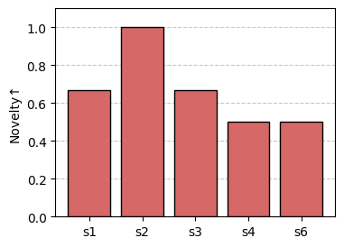
Notice missing values (e.g., “Novelty” for “s5”) are not shown in the barplot.

Caching

Discriminators and embedders can be computational expensive to execute. To reduce the number of function evaluations for these models, we can cache the results of discriminators and embedders.

The cache works like this: If a (sequence, embedding)-pair is already stored in the cache then retrieve the embedding. Otherwise compute the embedding, store the pair in the cache and retrieve the embedding.

Let’s create two toy models and the cache.

def my_embedder(sequences: list[str]) -> np.ndarray:
    lengths = [len(sequence) for sequence in sequences]
    counts = [sequence.count("K") for sequence in sequences]
    return np.array([lengths, counts], dtype=float).T


def my_discriminator(sequences: list[str]) -> np.ndarray:
    return np.ones(len(sequences)) * 0.85


cache = sm.Cache(models={"embedder": my_embedder, "discriminator": my_discriminator})

Optional: We can manually add model outputs to the cache. This is useful when e.g., (sequence, embedding)-pairs are already pre-computed and stored in a file.

seqs = ["MKQW", "AA", "BB"]
reps = my_embedder(seqs)

pairs = dict(zip(seqs, reps, strict=True))

cache.add(model_name="embedder", element=pairs)

Let’s compute the metrics. Since the metrics Precision, Recall, Clipped coverage, Clipped density use the same embedding model (embedder), the embedding is only computed once per sequence in sequences (instead of four times)!

Notice, we now use cache.model() instead of the embedder reference (my_embedder) directly.

df = sm.evaluate(
    sequences={
        "hyformer": ["RMKQW", "RKSPL", "RRRASD"],
        "HydrAMP": ["MKQW", "RKSPLP"],
        "Random": ["AAA", "PPPPP"],
    },
    metrics=[
        sm.metrics.Precision(
            reference=["AKWR", "AKKR", "KKKK"],
            embedder=cache.model("embedder"),
            n_neighbors=1,
            strict=False,
        ),
        sm.metrics.Recall(
            reference=["AKWR", "AKKR", "KKKK"],
            embedder=cache.model("embedder"),
            n_neighbors=1,
            strict=False,
        ),
        sm.metrics.ClippedDensity(
            reference=["AKWR", "AKKR", "KKKK"],
            embedder=cache.model("embedder"),
            n_neighbors=1,
            strict=False,
        ),
        sm.metrics.ClippedCoverage(
            reference=["AKWR", "AKKR", "KKKK"],
            embedder=cache.model("embedder"),
            n_neighbors=1,
            strict=False,
        ),
    ],
)

sm.show(df, color="#69bce8")

100%|██████████| 12/12 [00:00<00:00, 526.66it/s, data=Random, metric=Clipped coverage]  

	Precision↑	Recall↑	Clipped density↑	Clipped coverage↑
hyformer	0.67	0.00	1.00	0.67
HydrAMP	0.50	0.67	0.75	1.00
Random	0.00	0.33	0.00	0.00

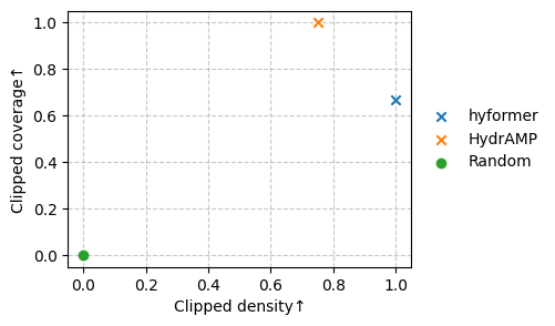
Let’s plot a scatterplot of the metrics.

metrics = ["Clipped density", "Clipped coverage"]
df = sm.rank(df, metrics)

markers = np.where(df[("Rank", "value")] == 1, "x", "o")
sm.plot_scatter(df, metrics=metrics, marker=markers)

Let’s write the cached (sequence, embedding)-pairs for each model to a file and reinitialize the cache.

PATH = "precomputed.pkl"

sm.to_pickle(cache.get(), PATH)

precomputed = sm.read_pickle(PATH)

cache = sm.Cache(init_cache=precomputed)
pprint(cache.get())

{'discriminator': {},
 'embedder': {'AA': array([2., 0.]),
              'AAA': array([3., 0.]),
              'AKKR': array([4., 2.]),
              'AKWR': array([4., 1.]),
              'BB': array([2., 0.]),
              'KKKK': array([4., 4.]),
              'MKQW': array([4., 1.]),
              'PPPPP': array([5., 0.]),
              'RKSPL': array([5., 1.]),
              'RKSPLP': array([6., 1.]),
              'RMKQW': array([5., 1.]),
              'RRRASD': array([6., 0.])}}

Tip: The cache can become very useful if you use an external tool to predict sequence properties, e.g., a command-line tool or a tool implemented in another programming language. Now you want to use these predictions in seqme to a compute metric. To do so, 1. read the predictions stored in a file and 2. pre-init the Cache with these (sequence, predictions)-pairs.

Creating a new metric

You can also integrate your own metrics into seqme through the Metric interface as shown below.

class MyMetric(sm.Metric):
    def __init__(self, amino_acid: str, minimize: bool = True):
        self.amino_acid = amino_acid
        self.minimize = minimize

    def __call__(self, sequences: list[str]) -> sm.MetricResult:
        aa_count = sum([seq.count(self.amino_acid) for seq in sequences])
        aa_total = sum([len(sequence) for sequence in sequences])
        return sm.MetricResult(aa_count / aa_total)

    @property
    def name(self) -> str:
        return f"{self.amino_acid}-frequency"

    @property
    def objective(self) -> Literal["minimize", "maximize"]:
        return "minimize" if self.minimize else "maximize"

Let’s use our new metric.

df = sm.evaluate(
    sequences={
        "hyformer": ["MKQW", "RKSPL", "RASD"],
        "HydrAMP": ["MKQW", "RKSPL"],
        "Random": ["AAAA", "PPPPP"],
    },
    metrics=[
        MyMetric(amino_acid="K", minimize=False),
        MyMetric(amino_acid="R", minimize=True),
    ],
)

sm.show(df, color="#e07fe1", color_style="bar", caption="Table 1. Our first metric 🎉")

100%|██████████| 6/6 [00:00<00:00, 2613.54it/s, data=Random, metric=R-frequency]  

Table 1. Our first metric 🎉

	K-frequency↑	R-frequency↓
hyformer	0.15	0.15
HydrAMP	0.22	0.11
Random	0.00	0.00

We have now covered the main functionality of seqme! 🎉

seqme also contains functionality to add third-party models, evaluate embedding models alignment with the property/properties of interest and a few extra things.