Diagnostics & Visualizations#
Recall embedding-based metrics rely on an embedding model. How do we choose a “good” embedding model for the biological sequences of our interest - so we can later evaluate these sequences with the embedding-based metrics? We will answer this question in this notebook. We will also show how to visualize embeddings using seqme.
import matplotlib.pyplot as plt
import numpy as np
import seaborn as sns

import seqme as sm
Embedding models#
Let’s start by loading some sequences.
DATASET_PATHS = {
    "UniProt": "./data/dbs/uniprot/uniprot_8_50_100.fasta",
    "AMP-data": "./data/dbs/amps.fasta",
}
datasets = {name: sm.read_fasta(path) for name, path in DATASET_PATHS.items()}
for model_name, sequences in datasets.items():
    print(f"{model_name}: {len(sequences)} sequences")
UniProt: 2933310 sequences
AMP-data: 38473 sequences
n_samples = 500
seed = 42

data = {
    name: sm.utils.subsample(sequences, n_samples=n_samples, seed=seed) if len(sequences) > n_samples else sequences
    for name, sequences in datasets.items()
}
Let’s setup the cache.
models = {
    "charge": sm.models.Charge(),
    "esm2": sm.models.ESM2(
        model_name=sm.models.ESM2Checkpoint.t6_8M,
        batch_size=256,
        device="cpu",
        verbose=True,
    ),
    "hyformer": sm.models.Hyformer(
        model_name=sm.models.HyformerCheckpoint.peptides_34M,
        batch_size=256,
        device="cpu",
        verbose=True,
    ),
}

cache = sm.Cache(models)
Model weights loaded from SzczurekLab/hyformer_peptides_34M
Model state_dict loaded with `strict=False`. Missing keys: [], Unexpected keys: ['prediction_head.dense.weight', 'prediction_head.dense.bias', 'prediction_head.out_proj.weight', 'prediction_head.out_proj.bias']
/Users/rasmus.larsen/work/hackathon-2025/seqme/.conda/lib/python3.11/site-packages/hyformer/models/utils/state_dict_utils.py:29: UserWarning: Model is not compiled but state dict is. Removing prefix from state dict.
  warnings.warn("Model is not compiled but state dict is. Removing prefix from state dict.")
Diagnostics#
We are interested in selecting an embedding model which orders the embedding space by “AMP”-likeness, i.e., the degree in which a peptides “looks” like a peptide with antimicrobial properties.
positives = data["AMP-data"]
negatives = data["UniProt"]

labels = np.array([0] * len(negatives) + [1] * len(positives))
sequences = negatives + positives
cache.add("esm2-4d", sm.models.PCA(cache.model("esm2"), sequences, n_components=4))
cache.add("hyformer-4d", sm.models.PCA(cache.model("hyformer"), sequences, n_components=4))
100%|██████████| 4/4 [00:06<00:00,  1.55s/it]
  0%|          | 0/4 [00:00<?, ?it/s]/Users/rasmus.larsen/work/hackathon-2025/seqme/.conda/lib/python3.11/site-packages/torch/utils/data/dataloader.py:692: UserWarning: 'pin_memory' argument is set as true but not supported on MPS now, device pinned memory won't be used.
  warnings.warn(warn_msg)
100%|██████████| 4/4 [00:18<00:00,  4.67s/it]
Feature alignment score#
To evaluate “AMP-likeness”, we can use the feature alignment score which is a measure for how homogenous neighborhoods are in the embedding space. We prefer AMPs cluster together. Thus, we compute the feature alignment score for different neighborhood sizes. A score of 1.0 means the sequences are clustered by “AMP-likeness”. A score of 0.0 means the embedding space is not able to group by our feature of interest.
n_neighbours = [1, 2, 4, 8, 16, 32, 64, 128]
embedding_models = ["esm2", "esm2-4d", "hyformer", "hyformer-4d"]

fig, ax = plt.subplots(figsize=(4, 3))
for model_name in embedding_models:
    xs = cache.model(model_name)(sequences)
    sm.utils.plot_knn_alignment_score(xs, labels, n_neighbours, label=model_name, ax=ax)
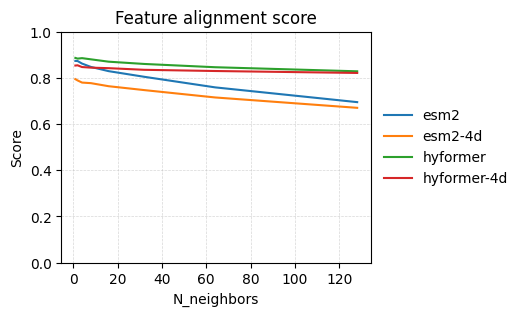
The sequences produced by hyformer is better at seperating AMPs from non-AMPs than the other.
Spearman alignment score#
The spearman alignment score computes how well an embedding space aligns with a reference embedding space. We know AMPs are usually positively charged, so let’s see how well the embedding model aligns with this feature.
xs_embedder_esm2 = cache.model("esm2")(sequences)
xs_charge = cache.model("charge")(sequences)

score = sm.utils.spearman_alignment_score(xs_embedder_esm2, xs_charge[:, None])

print(f"Spearman correlation coefficient: {score:.2f}")
Spearman correlation coefficient: 0.19
xs_embedder_hyformer = cache.model("hyformer")(sequences)
xs_charge = cache.model("charge")(sequences)

score = sm.utils.spearman_alignment_score(xs_embedder_hyformer, xs_charge[:, None])

print(f"Spearman correlation coefficient: {score:.2f}")
Spearman correlation coefficient: 0.10
Visualization#
Let’s now visualize the embedding spaces.
First let’s extract the sequences to visualize.
colors = ["red", "green"]

embedder_name_esm2 = "esm2"
embedder_name_hyformer = "hyformer"

embedder_esm2 = cache.model(embedder_name_esm2)
embedder_hyformer = cache.model(embedder_name_hyformer)
embeddings_esm2 = {name: embedder_esm2(sequences) for name, sequences in data.items()}
embeddings_hyformer = {name: embedder_hyformer(sequences) for name, sequences in data.items()}

embedding_names_esm2 = list(embeddings_esm2.keys())
embedding_names_hyformer = list(embeddings_hyformer.keys())

embedding_values_esm2 = list(embeddings_esm2.values())
embedding_values_hyformer = list(embeddings_hyformer.values())
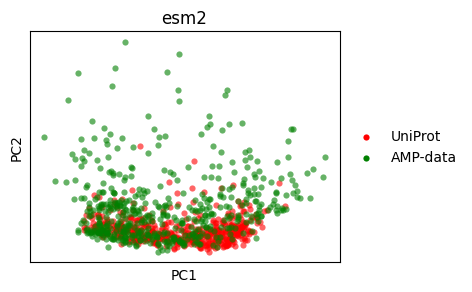
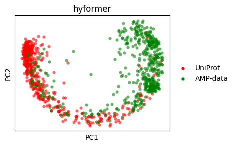
PCA#
Let’s do a PCA plot.
pca_esm2 = sm.utils.pca(embedding_values_esm2)
pca_esm2 = dict(zip(embedding_names_esm2, pca_esm2, strict=True))

pca_hyformer = sm.utils.pca(embedding_values_hyformer)
pca_hyformer = dict(zip(embedding_names_hyformer, pca_hyformer, strict=True))
sm.utils.plot_embeddings(
    pca_esm2.values(),
    values=pca_esm2.keys(),
    colors=colors,
    title=embedder_name_esm2,
    xlabel="PC1",
    ylabel="PC2",
)
sm.utils.plot_embeddings(
    pca_hyformer.values(),
    values=pca_hyformer.keys(),
    colors=colors,
    title=embedder_name_hyformer,
    xlabel="PC1",
    ylabel="PC2",
)
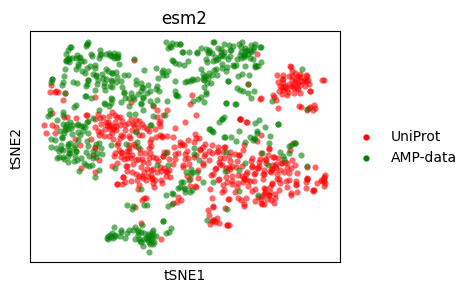
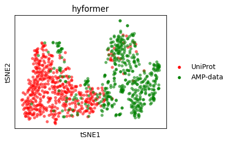
t-SNE#
Let’s do a t-SNE plot.
tsne_esm2 = sm.utils.tsne(embedding_values_esm2)
tsne_esm2 = dict(zip(embedding_names_esm2, tsne_esm2, strict=True))

tsne_hyformer = sm.utils.tsne(embedding_values_hyformer)
tsne_hyformer = dict(zip(embedding_names_hyformer, tsne_hyformer, strict=True))
sm.utils.plot_embeddings(
    tsne_esm2.values(),
    values=tsne_esm2.keys(),
    colors=colors,
    title=embedder_name_esm2,
    xlabel="tSNE1",
    ylabel="tSNE2",
)
sm.utils.plot_embeddings(
    tsne_hyformer.values(),
    values=tsne_hyformer.keys(),
    colors=colors,
    title=embedder_name_hyformer,
    xlabel="tSNE1",
    ylabel="tSNE2",
)
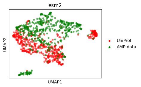
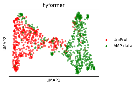
UMAP#
Let’s do a UMAP plot.
umap_esm2 = sm.utils.umap(embedding_values_esm2)
umap_esm2 = dict(zip(embedding_names_esm2, umap_esm2, strict=True))

umap_hyformer = sm.utils.umap(embedding_values_hyformer)
umap_hyformer = dict(zip(embedding_names_hyformer, umap_hyformer, strict=True))
sm.utils.plot_embeddings(
    umap_esm2.values(),
    values=umap_esm2.keys(),
    title=embedder_name_esm2,
    colors=colors,
    xlabel="UMAP1",
    ylabel="UMAP2",
)
sm.utils.plot_embeddings(
    umap_hyformer.values(),
    values=umap_hyformer.keys(),
    title=embedder_name_hyformer,
    colors=colors,
    xlabel="UMAP1",
    ylabel="UMAP2",
)
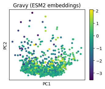
Embedding + Property#
Let’s do an UMAP for a single list of sequences and color those sequences based on a property.
property_model = sm.models.Gravy()

sm.utils.plot_embeddings(
    pca_esm2.values(),
    values=[property_model(data[name]) for name in pca_esm2.keys()],
    title="Gravy (ESM2 embeddings)",
    alpha=1.0,
    cmap="viridis",
    xlabel="PC1",
    ylabel="PC2",
)
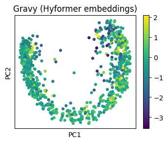
property_model = sm.models.Gravy()

sm.utils.plot_embeddings(
    pca_hyformer.values(),
    values=[property_model(data[name]) for name in pca_hyformer.keys()],
    title="Gravy (Hyformer embeddings)",
    alpha=1.0,
    cmap="viridis",
    xlabel="PC1",
    ylabel="PC2",
)
Property models#
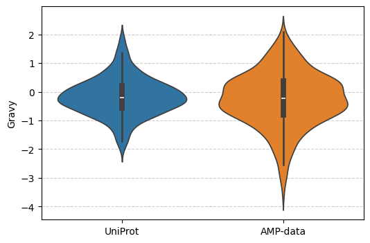
Let’s create a violin plot for one property.
cache = sm.Cache(models={"Gravy": sm.models.Gravy(), "Molecular Weight": sm.models.ProteinWeight()})
properties = {name: cache.model("Gravy")(sequences) for name, sequences in data.items()}
fig, ax = plt.subplots(figsize=(6, 4))
ax.grid(axis="y", linestyle="--", alpha=0.6)
ax.set_axisbelow(True)
ax.set_ylabel("Gravy")
sns.violinplot(properties, bw_method="scott", ax=ax)
<Axes: ylabel='Gravy'>